Completed Test: April 13, 2018
Originally we wanted to include an LCD into our project for the displaying the health state of the retina fundus image after is goes through the image processing through MATLAB. After discussing this with our advisors, we realize that the inclusion seems rather difficult and pointless due to the given time. Thus we used an LED as an indicator instead; the LED is attached on a breadboard and is accessed by MATLAB through the Raspberry Pi's GPIO Pins. So whenever the algorithm determines that the retinal image it sees has the disease, it will blink, when it sees that it doesn't have it, it won't blink.
Challenges:
The main challenge in this aspect of the project was to learn how to use MATLAB to access the GPIO pins of the Raspberry Pi 3. Hooking up the LED on a bread was plain and simple, connecting it to the pins of the Raspberry Pi required some research on the Internet to know which pins exactly were needed to be selected, while knowing how to program LEDs to flash on and off required some programming and research.
The procedure in getting this portion to work goes as:
1. Finding a breadboard, some jumper wires, and an LED
2. Research which pin numbers matched to the pin values that MATLAB reads
3. Connecting the LED on breadboard to two GPIO pins of the Raspberry Pi 3, with one pin connecting a power-based pin and the other connected to ground-based pin
4. Use MATLAB to program with GPIO pin would supply current, if statements and commands related to the support package were used to make this work
if strcmp(answer, 'DiabeticRetinopathy')
configureDigitalPin(mypi,14,'output')
writeDigitalPin(mypi,14,0)
else
writeDigitalPin(mypi,14,1)
end
5. Run the simulation and the LED should light up depending on the condition
Results: April 13, 2018
Results:
From the test, the LED is now able to light up whenever the algorithm from MATLAB detects retinal image to be Diabetic Retinopathy and that it will not blink whenever the algorithm detects the retinal image to be Healthy. So basically when the output of the algorithm equals "DiabeticRetinopathy" a one/on value is sent to the GPIO pin connected to the positive terminal of the LED and supplies a voltage of 3.3V into it thus enabling it to blink or light up. When the algorithm equals "Healthy", a zero/off value is sent to the GPIO pin connected to the LED and does not supply any voltage.
From the test, the LED is now able to light up whenever the algorithm from MATLAB detects retinal image to be Diabetic Retinopathy and that it will not blink whenever the algorithm detects the retinal image to be Healthy. So basically when the output of the algorithm equals "DiabeticRetinopathy" a one/on value is sent to the GPIO pin connected to the positive terminal of the LED and supplies a voltage of 3.3V into it thus enabling it to blink or light up. When the algorithm equals "Healthy", a zero/off value is sent to the GPIO pin connected to the LED and does not supply any voltage.
Completed Test: April 10, 2018
April 10 2018
After installing Raspbian on the Raspberry Pi and connecting and using the camera by installing the camera software, the next step forward was to get the SBC connecting to the Pi in order to access the microcontroller and its camera using MATLAB. With the connection, we would be able to utilize the camera from the Pi to take a picture a retina fundus photograph where that will be sent to the SBC where MATLAB will read, process, and detect whether the picture contains patterns of Diabetic Retinopathy or not.
Challenges:
The challenge is this procedure was to know how to connect the SBC connected to the Raspberry Pi 3 properly. This was done before when our Raspberry Pi's OS was Ubuntu Mate, but now we are using Raspbian.
How this procedure of the project was accomplished was through a small amount steps involving both hardware and software applications
1. Connect a USB-Ethernet adapter to the Raspberry Pi 3.
2. Connect straight-through Ethernet Cable from adapter to Raspberry Pi 3.
3. Create a connection from MATLAB to pi using the command : mypi = raspi.
4. Test connection using MATLAB commands such as : writeLED and system.
Results: April 10, 2018
Results:
The SBC containing MATLAB programming application now has connection with the Raspberry Pi 3 and can access the microcontroller through various commands. It's able to access the camera and enable it to take pictures through the snapshot command, it's also able to see the pictures that the camera takes and use it for its functional purpose.
The SBC containing MATLAB programming application now has connection with the Raspberry Pi 3 and can access the microcontroller through various commands. It's able to access the camera and enable it to take pictures through the snapshot command, it's also able to see the pictures that the camera takes and use it for its functional purpose.
Completed Test: April 6, 2018
April 6, 2018
The reason for the test is that we can work with an Operating System that has better compatibility with the MATLAB support packages for the Raspberry Pi. It's also the default OS of the Pi, thus made it easier for us to attain assistance from the Jnternet and other peers.
Challenges:
At first our operating system was Ubuntu Mate, but after having issues in installing the MATLAB support packages for out Raspberry Pi we decided to switch our operating system, to Raspbian since it is the default operating system for our Pi and MATLAB. The major challenge with this part was in installing and working with an operating system for the Raspberry Pi that we’d never used before.
- To install Raspbian, a new SD (secure disk) Card must be used in order to flash the image onto it. Our card was a SanDisk 16G SD (secure disk) Card.
- The application used to flash the Raspbian is Etcher thus the first step was to download the application.
- The zip file of Raspbian from the Raspberry Pi’s official website had to be downloaded.
- Using an extraction application, 7-zip, was used to extract the image file out of the folder.
- After inserting the SD (secure disk) card into the PC without formatting it, Etcher was then used to flash the Raspbian image into the hard drive. This process took about 20 minutes.
- When the process was completed, the SD (secure disk) card was inserted into the Raspberry Pi and after manually connecting the required components to power the device, our new operating system was able to boot.
- With a new operating system, the camera software had to be installed again and that was done through the same procedures done through Ubuntu Mate.
- A major challenge in using Raspbian as our operating system was to prevent the SD (secure disk) card from being corrupted after shutting down each time. This was fixed after downgrading the resolution of the OS, it was changed from the default size to CEA Mode 2 720x480 60Hz 4.3.
Results: April 6, 2018
The result of this is now Raspbian Operating System and SD (secure disk) Card drive are now stable and free from corruption. With it, we can now boot our Raspberry Pi and the Operating System smoothly without issues.
The RaspbianOS is the operating system most usable and supported by the Raspberry Pi 3 Model B.
Completed Test: April 1, 2018
April 1, 2018
This test was to use the ArduCAM to take an image with the Raspberry Pi3 Model B. This test will help us in the next aspect of the project where we use MATLAB on the raspberry pi in order to take an image of a retinal fundus image using the ArduCAM.
Challenges:
One challenge to tackle in the hardware aspect was to connect our camera to the Pi in order to use it to take pictures of retina fundus images, and be sent to the Raspberry Pi Model 3B for image processing. After correctly connecting the camera, Raspberry Pi, and using the right Terminal commands to access it, an error arose saying that the camera was not detected thus another challenge was to troubleshoot this error in order for the camera to work properly.
Initially we interfaced the Arducam, the type of camera used, to our Raspberry Pi with the operating system of Ubuntu Mate
- Connected the camera by attaching the camera’s wires to the ISP of the Raspberry Pi.
- Boot the Raspberry Pi into it’s Operating System, Ubuntu Mate.
- Open the system’s settings using sudo raspi-config.
- An error occurred where Terminal said it didn’t recognize the command. The issue with this is that we needed to install configuration settings of Raspberry Pi for the operating system. The command to do this was sudo apt-get install raspi-config rpi-update.
- Now from using the sudo raspi-config, the Pi’s configuration menu opens up listing options for the user to configure.
- Select Enable Camera option, select yes for enabling camera, and then reboot.
- Another error occurred stating the camera was not detected. After searching for some intel on the net, we realized that certain changes must be made on the Pi’s boot/config.txt file. The two commands were: start_x=1 gpu_mem=128.
- From using the command raspistill -o image.jpg, the camera had successfully taken a photo.
Results: April 1, 2018
The result of this is that the camera is now interfaced with Raspberry Pi and the users, as we can now take photos using the terminal command.
This is an image that was taken with the ArduCAM on the raspberry pi, proving that it is possible to use it to take an image with an external camera.
Completed Test: March 28, 2018
March 28, 2018
In this test we automated taking pictures, saving them and testing them with our algorithm. So we were able to take images using an external camera in MATLAB, choose a name, file type and location to save the image. Then used the name and location of the image to test to see whether or not the image has diabetic retinopathy.
Challenges:
The first challenge that we faced was making sure we chose the right camera, file location and file name. Without these being carefully addressed we would be unable to get the picture to be taken. The next phase we had to figure out was how to get the for loop to end so that we could disengage the camera after it had been used.
1. Set a counter outside of my for loop.
2. Use the saveas function to choose the name that you want to save it as and location.
3. Increase the counter by one.
4. Use an if statement that sets the count as less than two, continue else end.
5. After use clear function to clear cam which allows us to clear the camera that was just used.
6. Use the imread function to select the folder read from and the file name.
7. Then use the predict function to predict whether the image is Healthy of has Diabetic Retinopathy.
8. We then show the Label the image received so it lets us know what group it was under.
Results: March 28, 2018
So, from this test we were able to conclude that we could take an image, automatically save it, test it, and display the results in a matter of seconds.
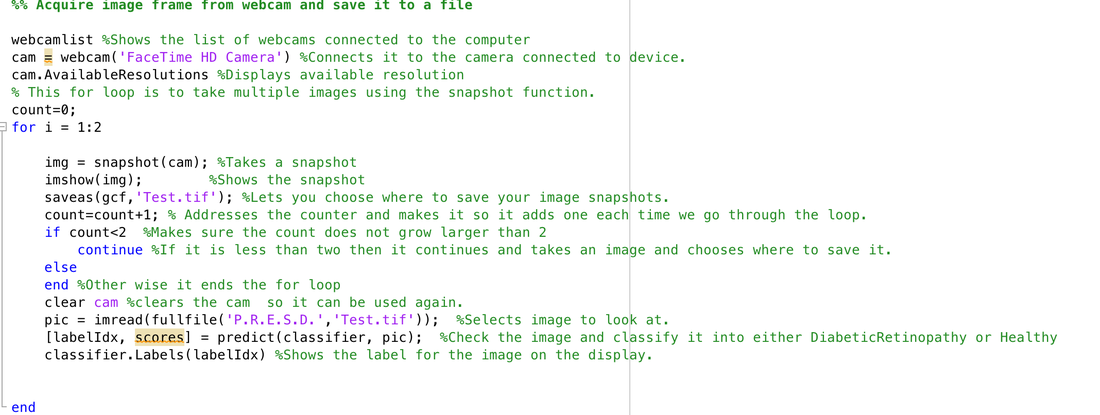
This is the code that was edited in order to get our program to take the images. We had to add in an if statement, and utilize a counter to get the code to run properly and produce an accurate result. After the if statement we were able to select a file to test, had our algorithm make the prediction and show the label it gave the image in the display window.
Completed Test: March 7, 2018
March 7, 2018
In this test we tested 60 different images. 30 were images with diabetic retinopathy and 30 were images of healthy retinas. We then took our results, calculated the accuracy of both types and found the average accuracy between the two groups.
1. We ran 30 images of healthy retinas through our algorithm, which resulted in 25 correct results and 5 incorrect results.
2. We then found the percentage of correct results which was 83%.
3. We next ran 30 images of retinas effected by diabetic retinopathy through our algorithm, which resulted in 29 correct results and 1 incorrect result.
4. We then found the percentage of correct results was 97%.
5. We then added up all of the correct results in both groups, and found that we had 54 correct answers and 6 incorrect answers.
6. We then found the average percentage of correct results was 90%.
Results:March 7, 2018
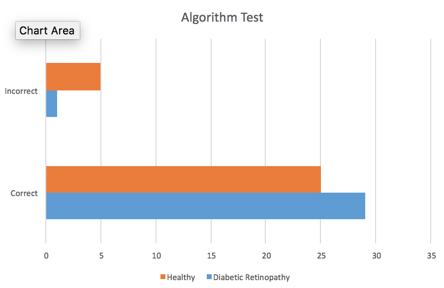
This bar graph represents the total number of correct images for Diabetic Retinopathy and Healthy, versus the number of incorrect images.
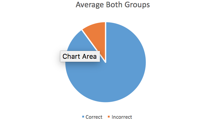
This pie graph represents the total number pf correct outcomes versus the total number of incorrect outcomes.
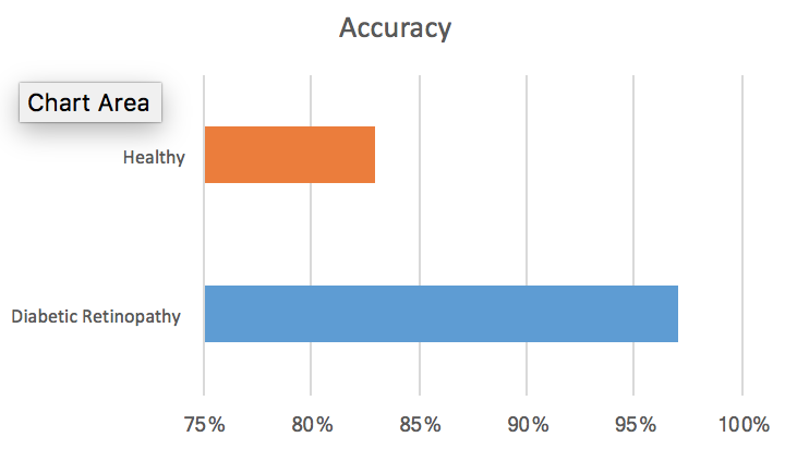
This bar graph shows the average accuracy of healthy retinas which was 83%, versus the average accuracy of diabetic retinopathy which was 97%.
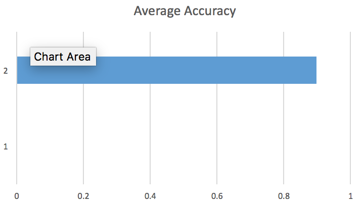
This bar graph shows the average accuracy of both groups which was 90%.
Completed Test: March 1, 2018
March 1, 2018
In this test we were able to take a photo of a retina, take a picture of it with the computer, store the image, and then run it through our code and get accurate results.
Challenge:
The big challenge we faced during this test was making sure the camera was taking a straight and clear shot of the image in order to get the most accurate result. There wasn't a big delay between photos so you have to be able to accurately and quickly.
1. So, we first take an image to test and make sure our camera is functioning properly.
2. We took a second image of the images we have which are test pictures that we know have diabetic retinopathy.
3. We then stored the image in a file.
4. We then ran the image file in the code to test for diabetic retinopathy.
5. The program then displays the category that it thinks the image is part of.
Results: March 1, 2018

This code we used in order to test the image we took with the camera and see if the algorithm would categorize it correctly.
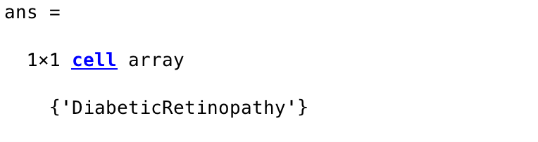
From this it told us that our image has diabetic retinopathy, which was an accurate result, and we were able to see this result from just my computer's camera.
Completed Test: February 21, 2018
February 21, 2018
In this test we were able to take an outside image, test it for diabetic retinopathy, and get the correct result.
Challenge:
The biggest challenge we had during this test was setting up the correct image path in order to access the image we wanted to test. Then the other issue was making sure we used the correct classifier in order to get an accurate result.
1. First, we had to use the imread function in order to select the image we want the program to read.
2. We next used the predict function in order to utilize our classifier and classify the image we acquired in our program.
3. We then used the label command in order to display the label given and to determine whether on not we were given the correct output from our algorithm.
4. In our case we gave it an image that we knew had diabetic retinopathy and it gave us the correct result at the output.
Results: February 21, 2018

This is the code we used on order to select the image, check the image and classify it, and display the result.
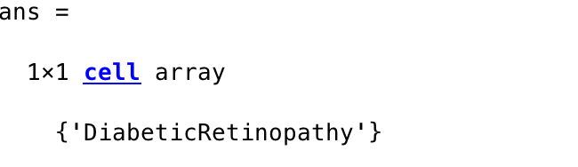
This is the result I received from the test image, which was diabetic retinopathy, and was the correct result.
Completed Test: February 15, 2018
February 15, 2018
In this test we were able to take an image using an external camera and send it to a folder.
Challenge:
We had a few different challenges during this test. The first one was getting the correct toolbox so that we could access the webcam using MatLab. The next issue we had was using the snapshot command and getting the camera to focus, we realized we would have to take more than one image in order to get the results we wanted. The next was saving the image and putting it in the correct folder took some time, but once completed was a simple task.
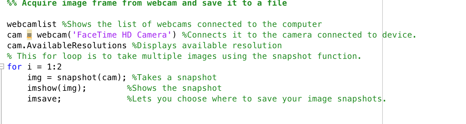
1. First we utilized the webcam list command to find out what cameras are connected to the device running the program.
2. Next we utilized the webcam command and set it to the camera we wanted to use to take our images.
3. After that we checked for the available resolution of the camera so we could see what type of image we would be able to take with the camera connected.
4. We then created a for loop.
5. Inside the for loop we used the snapshot command to take pictures using the camera we selected.
6. Next, we used the imshow command so that we could see what image the camera was taking and decide what is usable.
7. Finally we used the imsave command to choose a location to save the image and what to label it as.
In this test we were able to take an image using an external camera and send it to a folder.
Challenge:
We had a few different challenges during this test. The first one was getting the correct toolbox so that we could access the webcam using MatLab. The next issue we had was using the snapshot command and getting the camera to focus, we realized we would have to take more than one image in order to get the results we wanted. The next was saving the image and putting it in the correct folder took some time, but once completed was a simple task.
1. First we utilized the webcam list command to find out what cameras are connected to the device running the program.
2. Next we utilized the webcam command and set it to the camera we wanted to use to take our images.
3. After that we checked for the available resolution of the camera so we could see what type of image we would be able to take with the camera connected.
4. We then created a for loop.
5. Inside the for loop we used the snapshot command to take pictures using the camera we selected.
6. Next, we used the imshow command so that we could see what image the camera was taking and decide what is usable.
7. Finally we used the imsave command to choose a location to save the image and what to label it as.
Results: February 15, 2018
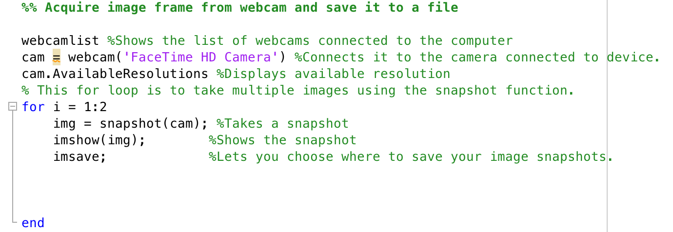
This is the code that was used in order to, check for the webcams, connect to the camera, check for resolution, take pictures with camera, show the image, and save it.
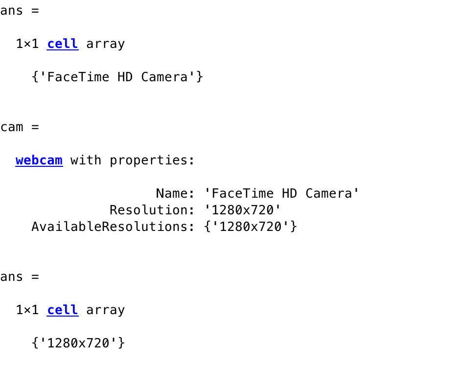
This image shows the results from running the above code.
Completed Test: February 8, 2018
February 8, 2018
In this test we eliminated the glaucoma group and increased the number of images in the algorithm in order to increase our accuracy.
Challenge:
The main challenge we faced during this test was getting our accuracy up to over 90% and making sure we get the most accurate results possible.
1. First we deleted the glaucoma part of our program in order to increase our accuracy. Sadly it only increased to around 80%, so we were not at our target goal.
2. Next we added more images to the DiabeticRetinopathy folder to increase the accuracy to over 90%.
3. When we increased the amount of photos to 45 in the folder, we found that we could get our Linear SVM accuracy to 91.7%.
Results: February 8, 2018
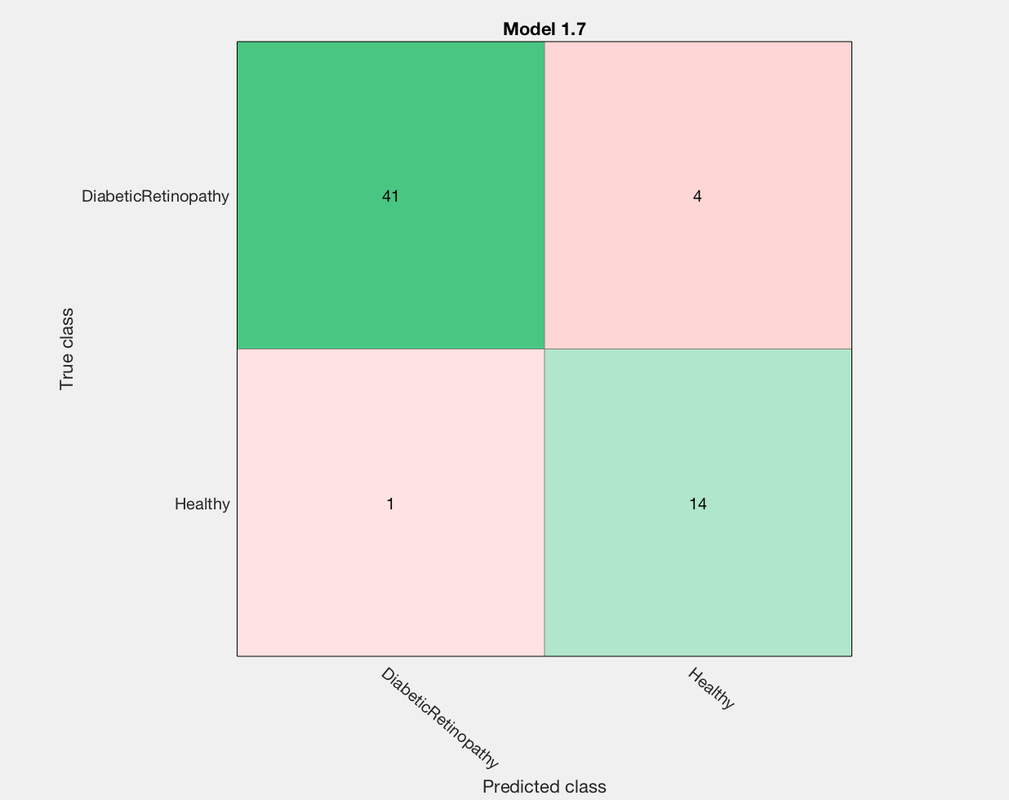
This is the confusion matrix I received once I got the Linear SVM accuracy to 91.7%.
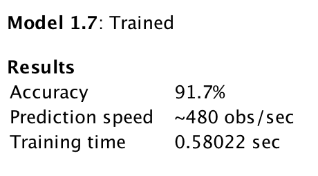
These are the results from training the Linear SVM which include the accuracy, prediction speed, and training time.
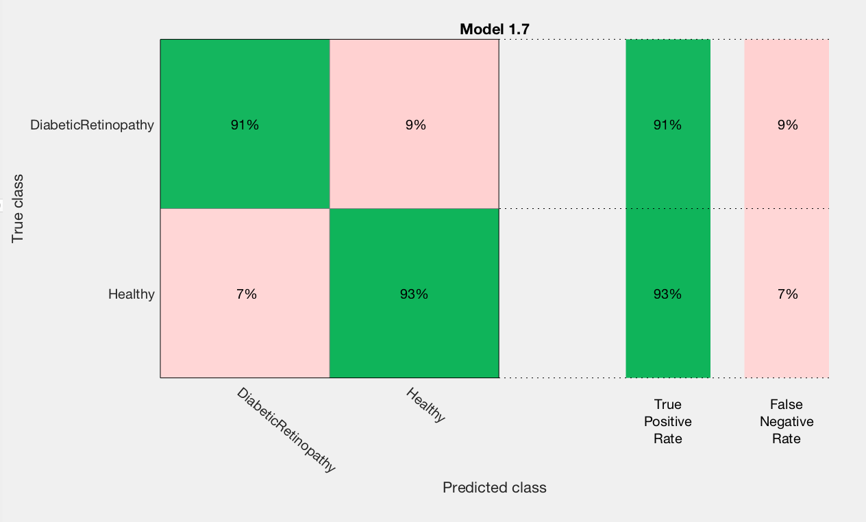
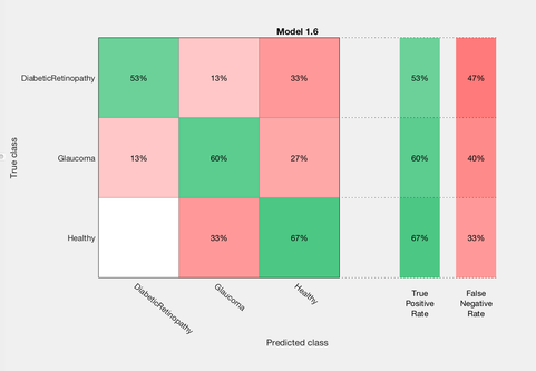
This is the part of the confusion matrix that shows the true positive rate and false negative rate. Both are above 90% accurate.
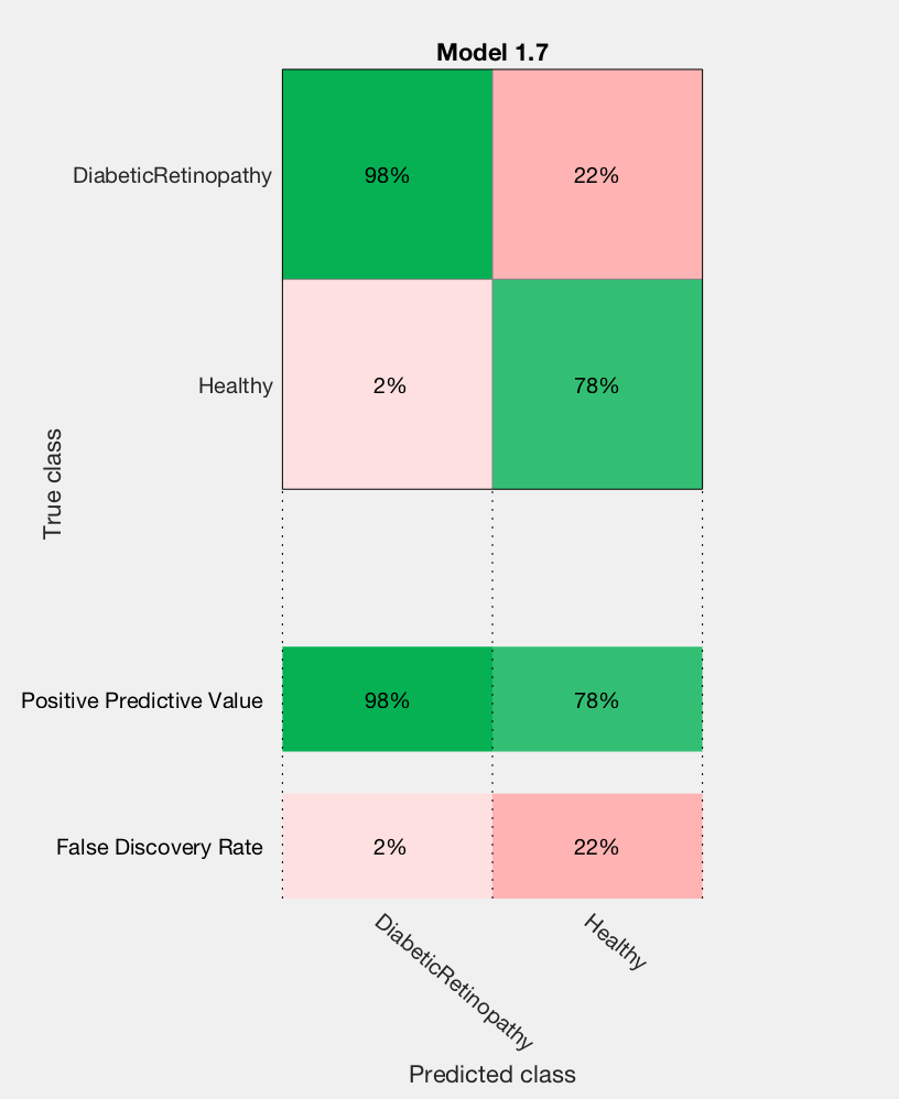
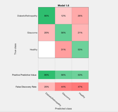
This is the part of the confusion matrix that displays the positive predictive value and the false discovery rate.
Completed Test: February 1, 2018
February 1, 2018
We tested different types of classifiers to determine which classifier would give us the highest accuracy, use minimal time, and perform the best in all three categories that we are testing.
Challenge:
The challenge we faced during this part of the project was using Classification Learner because we had never used this application previously, and it was hard to understand what needed to be tested initially and what the file would be named as.
1. First we had to run our machine learning algorithm, set up the bag of features and initialize the files we would be utilizing in the Classification Learner.
2. We ran Classification Learner in the program and made a new session by picking the correct file from the Workspace.
3. We started to train the classifiers by selecting all, and putting each classifier into their own individual Confusion Matrix.
4. Once each classifier was trained we were able to see the accuracy of each classifier, and put them into a table. The highest accuracy we received was 60%.
5. Eight different classifiers had this level of accuracy so we had to do more comparison tests.
6. We then looked at the Positive Predictive Values and the False Discovery Rates, to find the percentage of false positives.
7. After, we looked at the True Positive Rates and False Negative Rates, in order to see the summary of true values in each class.
8. From all of these different tests we were able to conclude that the Linear SVM Classifier was best suited for our project.
Results: February 1, 2018
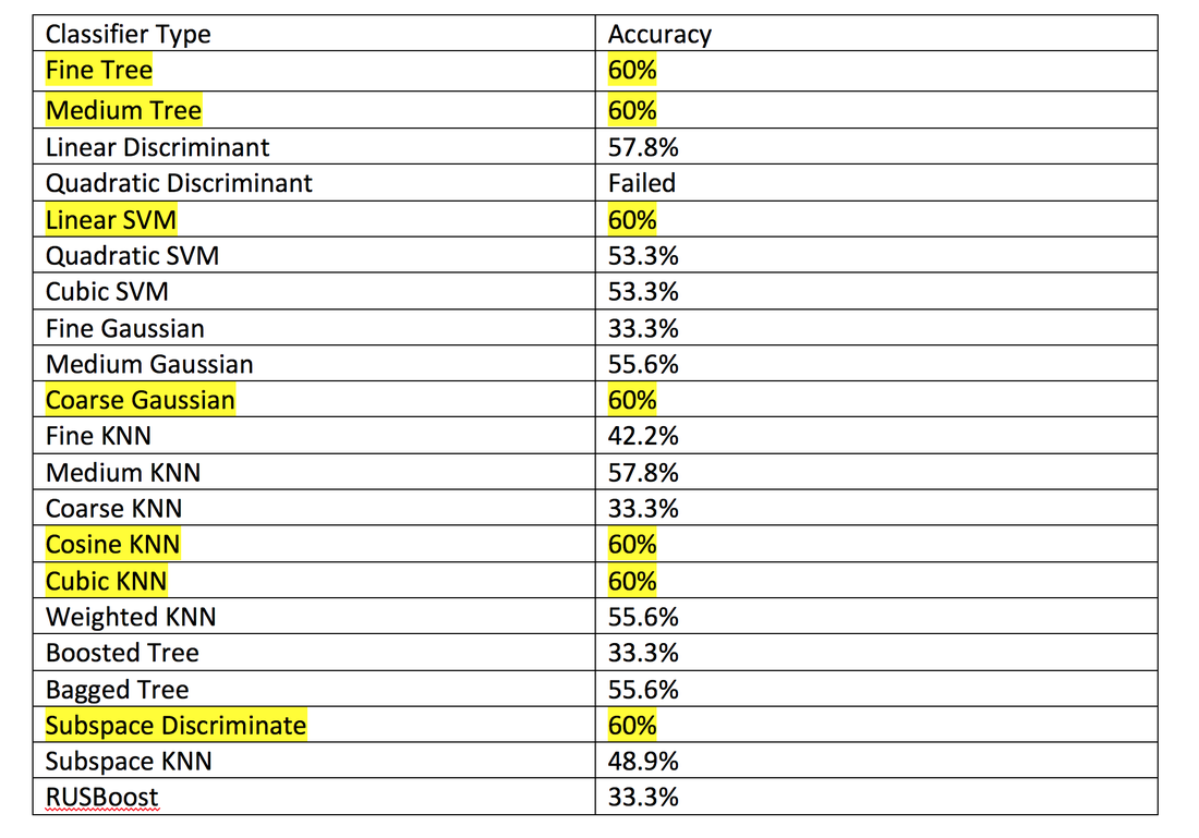
This is the table we created in order to see the accuracy of each type of classifier, and concluded that eight of them had the same high accuracy, so we would need to do more testing. These results were given by the Classification Learner Application by utilizing the Confusion Matrix.
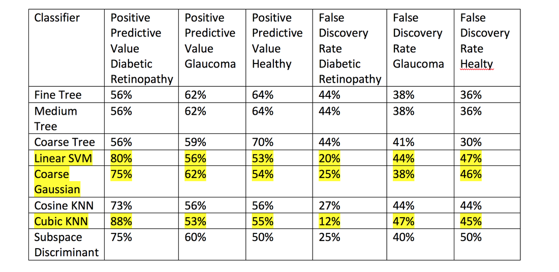
In this table we looked at the Post Predictive Value and False Discovery Rate of the eight most accurate classifiers and were able to conclude that the three with the highest prediction values are: Linear SVM, Coarse Gaussian, and Cubic KNN.
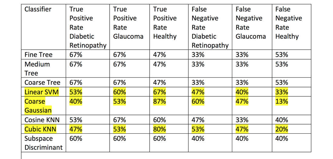
In this table we looked at the True Positive Rate and False Negative Rate of the eight most accurate classifiers, and were able to conclude that Linear SVM would be the most useful and accurate classifier for our project.
|
|
These two images represent the Linear SVM and the values that we received from training the classifier.
Completed Test: January 25, 2018
January 25, 2018
We were able to begin to use Matlab to develop our first machine learning algorithm.
Challenge:
We initially faced a large challenge which was using large sets of images, because it takes a lot of time and data in order to run through this algorithm.
1. We first saved all of our files and images inside of our P.R.E.S.D. folder, and inside the folder we had another folder called RetinaImages that contained the folders with images of Healthy, DiabeticRetinopathy, and Glaucoma eye scans.
2. Second, we labeled our image set which is a 1x3 matrix, and initially contained 45 images from three different class.
3. Third, we created a bag-of-features that selected 80% of the strongest features from the photos. Formed them into various clusters, and initialized and completed the clusters.
4. Fourth, we encoded diagrams, which had a visual representation of each retina type, and paired it with a graph that displayed the visual occurrences and frequency of these occurrences.
5. Fifth, we trained the image classifier (SVM) for each category , and then evaluated it in order to test the classifier.
6. Sixth, we evaluated our image classifier and found that our average accuracy is at 67%.
7. Seventh, we ran the prediction test, tested a random image in our files. The result came out correctly and occurred in less than a minute.
Testing Conclusions:
From this test we concluded that we will have to try different classifier types to see which one gives the most accurate results. Also, we will need to increase the amount of pictures in our algorithm in order to make it more reliable.
Results: January 25, 2018
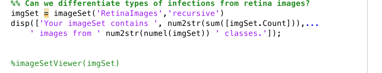
This code is used to grab images from inside of the folder called RetinaImages and categorize them into 3 different classes.
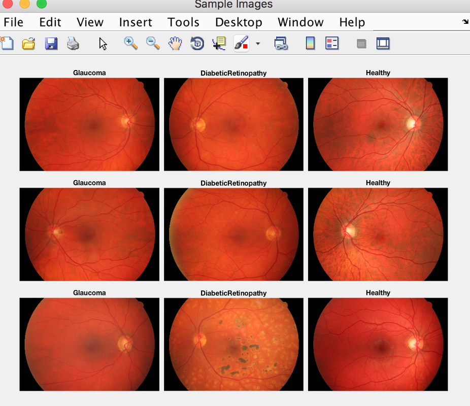
This window displays a group of sample images and groups them based off of the file they are stored in.
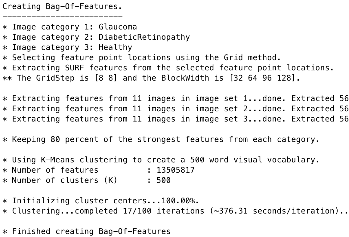
We, created the bag of features which looks at specific features for each image to determine how it should be classified.
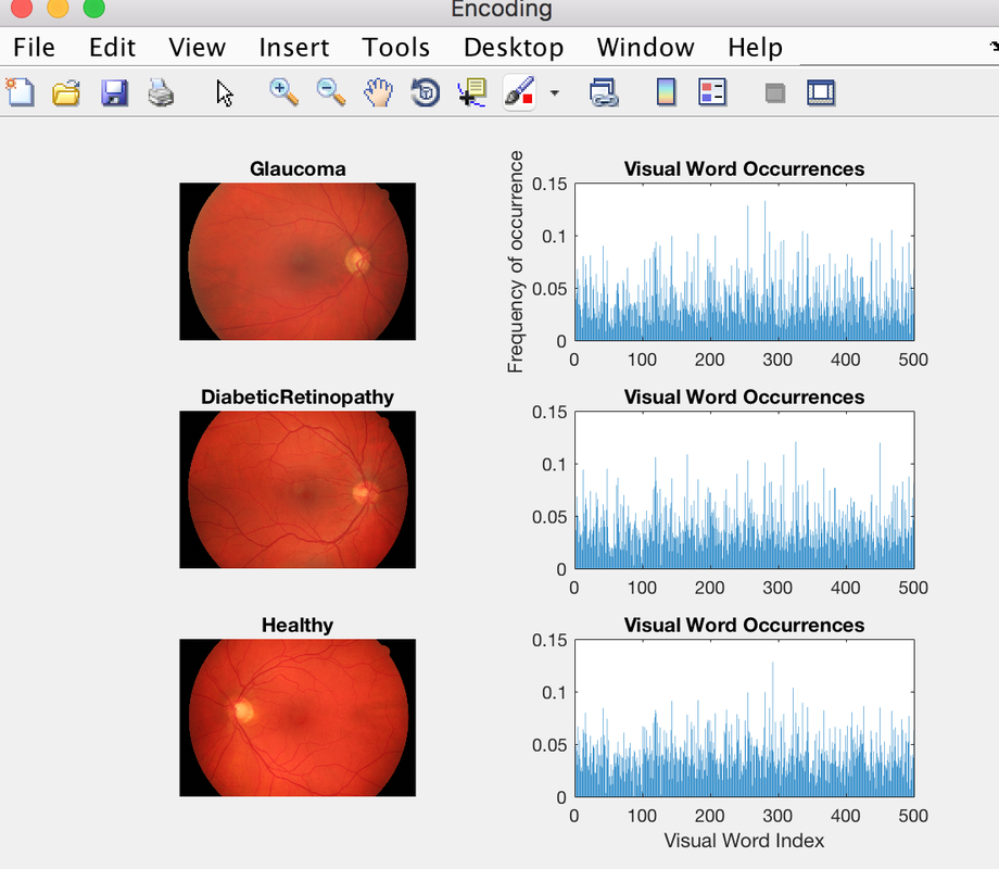
This window displays each group of images, and a graphical representation of the frequency of the visual occurrence.
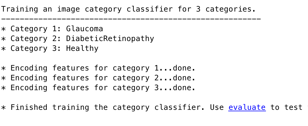
The results from training the classifier for all 3 categories.
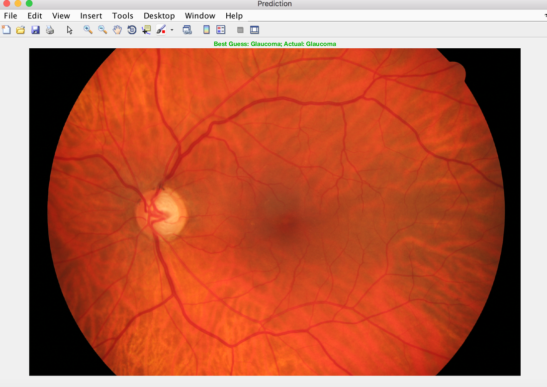
This Image, is one of a prediction being done about the image and is able to display the correct result at the top of the screen.
